Creating legible Excel formulas is something which is very handy, typically. No matter whether another person or oneself needs to adopt and understand an Excel file. It can be difficult to find into the logic of an old or alien Excel file: Then even plain calculations can be hard to grasp. But there are also cases where complex workbooks are easy to understand. It depends, as always:
Imagine a classical way to make an Excel file hard to understand: Adding numerous references across worksheets to single cells. This happens quite often. Even to adapt Excel users: For example, they separate calculation sheets from a parameter sheet. Conceptually, this is a good idea, but things can get messy.
Classical approach: Linking parameters directly
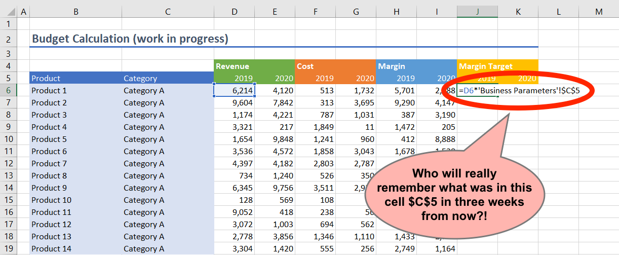
Consider the following case: A proper “Business Parameter” worksheet was set up. It contains lots of information (i.e. parameters). These will be required throughout the workbook.

Imagine a sheet “Budget Calculation” which needs certain parameters such as “Margin Target (%)”. In the formulas below, all parameters are referenced directly, e.g. via ‘Business Parameter’!$C$5. This is definitely correct, but who memorizes all these parameter references and addresses?! There might be dozens or even hundreds in complex Excel models. On top of this: Such formulas are both hard to read and to validate.
Named Range approach:
Named ranges are a reasonable approach to improve legibility. A named range can be used to give names single cells, whole ranges and even formula-based dynamic ranges. This means: In our business parameter worksheet every parameter needs to have its own name. For example:
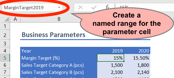
Writing the formula using a named range is straight forward: Just replace the absolute address ‘Business Parameter!’$C$5 with its name MarginTarget2019:

This is still correct and improves legibility tremendously. However, if there are too many parameters, it will take lots of time to create and maintain all required named ranges.
Excel Table approach #1
When trying to improve the Named Range approach from above, the legibility must not be harmed. It should be an approach which is legible, easy to maintain and simple to use. Fortunately, Excel tables offers all these characteristics when using a simple trick. First of all: An Excel table is not a worksheet. Some people might mistake the terms, anyway. An Excel table is a special kind of range with many great features. Instead of putting data and formulas somewhere on the worksheet it goes into an Excel table. One of its strength pays off when referencing columns in the Excel table: Table name and column name will be used instead of absolute ranges. For example “=ProductList[Sales 2013]” where “ProductList” is the table name and “Sales 2013” the column header. This formula references all cells in the “Sales 2013” column let it be 100 or 100,000 cells. Or just 1 cell.
An Excel table which has exactly one row behaves basically like a collection of single-cell named ranges. This makes it perfectly suited for the business parameter case here.
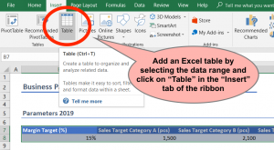
First of all, the parameters need to be brought into row-wise alignment:
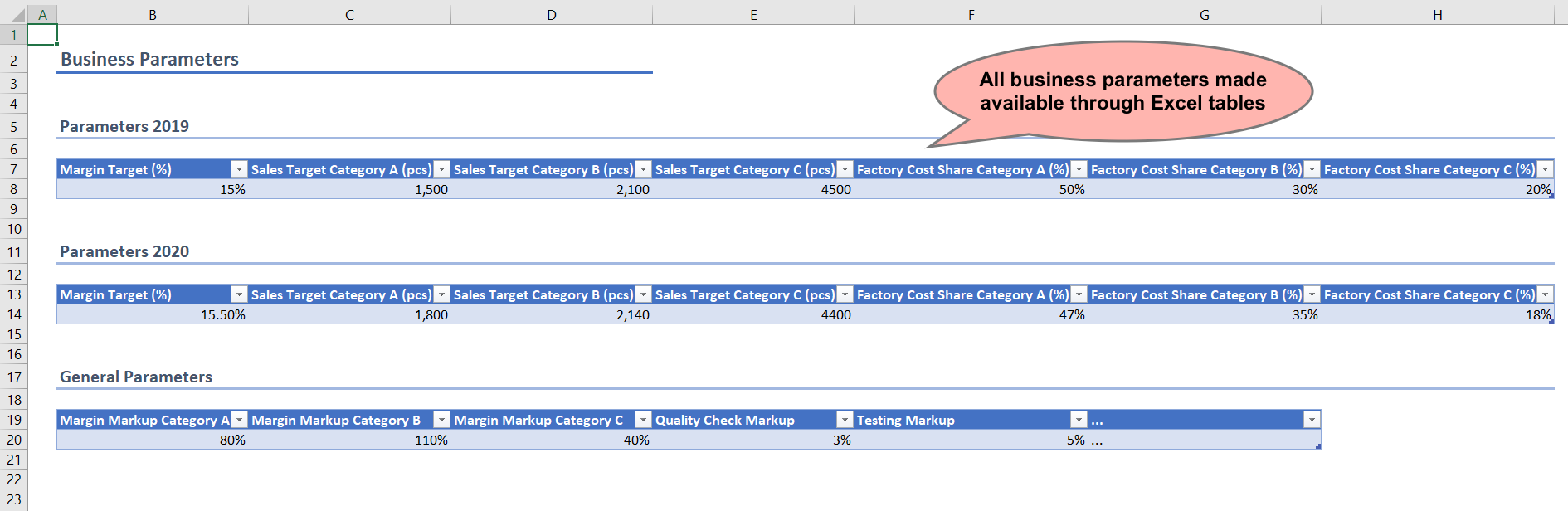
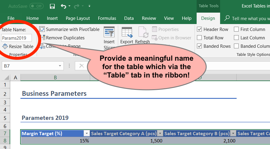
This screenshot contains already Excel tables which were created in the following way:
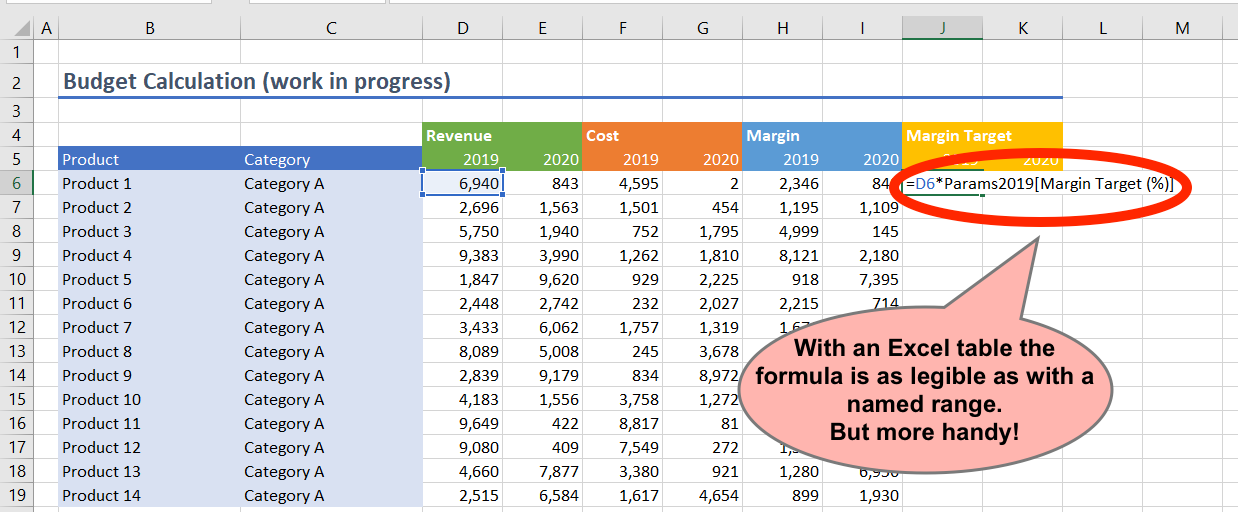
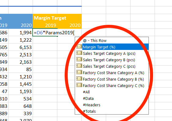
In the Budget Calculation worksheet the Excel table references will be used as parameter in the formula:
Excel Table approach #2
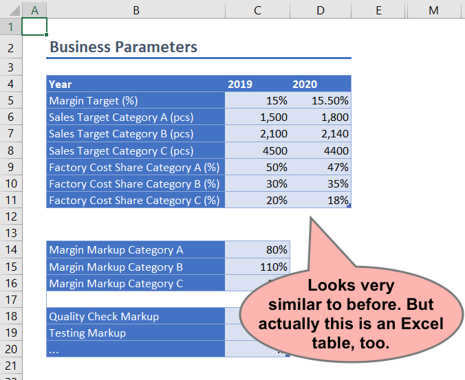
The first approach is very helpful. But it also leads to a different parameter sheet: It holds all data in rows instead of columns. Sometimes this is not the way to go. To keep the original idea of the parameter worksheet, this approach goes beyond #1. The difference will have no impact on the Budget Calculation. It only affect the business parameter worksheet. Consider the following screenshot, which contains the original parameter area and Excel tables side-by-side.

Of course, users shall not enter every parameter twice. For keeping the original layout and offering Excel table functionality, these parameters need to be a looked up. With an Index-Match formula, no cell-specific references are necessary. As a side note, a VLookup work as well but is nothing which I’d like to recommend.

Please note: For convenience and a more legible Index-Match formula, user parameter ranges were converted to Excel tables as well.
Another benefit when using Excel tables is the automatic dropdown. When writing formulas table names and column names are proposed. This is another discipline where Excel tables are at least as handy as named ranges.

Summary
It is not hard to create complex Excel models. However, it is challenging to make complex models legible and maintainable. The approach shown here helps to avoid absolute references to parameter worksheets. The recommendation is to use an Excel table which offers named referencing just like named ranges but with less effort to maintain. The idea is to restrict the Excel table to only one row such that referencing the whole column is actually referencing a mere cell.